Common wisdom says that running attracts a specific type of personality; independent, persistent, and with a masochistic streak. Having run with all different kinds of individuals over the past fifteen years, however, I deny this categorically; all kinds, all types I have encountered in my daily travels under the sun. Running attracts a mongrel variety of souls, drawn to the democratic nature of running which compels them all to suffer impartially.
Maybe that is why I began my first runs. Alone, out in the fields on the southern edge of Grand Forks, where after you emerged from the thinning treelines there was nothing save fallow fields and flat country cut squarewise by gravel roads, the emptiness of it and the silence of it suggestive of some terrible vastation. Out there on those leveled plains one could feel the wind blow uninterrupted from its travels from some unknown corner of earth and the sun burning into the cracked clay below, nothing out there beyond a few isolated rampikes and a distant horizon where sky bleeds into ground and faraway thunderclouds explode soundlessly.
As the years passed I continued to run and along the way I encountered all manner of runners. I ran with a thin, dark Indian chemist imported from the Malabar coast, and a stocky bruiser from Crawfordsville who, once he heaved his vast bulk into motion, appeared to move solely by momentum. I ran through the forested switchbacks of Paynetown with an erudite librarian from Tennessee and a halfwitted pervert from Elletsville who expectorated thin lines of drool whenever he talked excitedly. I ran a hundred-mile relay in the dead of night accompanied only by a black man with an emaciated form and a head that bobbed wildly as he jogged and an indoor track athlete whose body was adorned with all matter of piercings and gemgaws and a tattoo of an anatomically correct heart stenciled into his left breast.
I ran with an insomniac exhibitionist who, in the brain-boiled delirium of his restless nights, would arise and run through campus clad in his shoes only and only once did he ever encounter someone, and that man probably mistaking him for some kind of crazed phantom. I ran with a pair of gentlemen from Michigan passing through Bloomington who seemed to revere running as some kind of aristocratic sport and I ran with a curlyhaired dwarf of a man from New Hampshire whose friend had suffocated under an avalanche and I ran with an old ultramarathon veteran from Ohio with lymph pooling in his legs and the joints of his knees encrusted with grout who reckoned he'd been running on his feet longer than I had been alive. I ran with a confirmed vegetarian from Rhode Island who spoke fondly of the days when there were no mounts and there were no weapons to adulterate the sacredness of the hunt and animals were run to the outermost limit of exhaustion whereupon their hearts burst silently.
Above all, I ran by myself. I ran through hail the size of grapes and I ran through thunder loud as a demiculverin next to your ear and I ran through heat and humidity seemingly designed to instill craziness into its victim. I ran down valleys of emerald grass and I ran up bluffs fledged with dying trees and I ran through dried gulches, my barkled shoes carrying clods of earth far away from where they were meant to be. I ran down all manner of roads, lanes, boulevards, avenues, trails, and paths. I ran during the meridian of the day and I ran in the inky blackness of the early morning where only the traffic lights showed any animation in their monotonous blinking and I ran until my clothes were rancid and my socks vile and my skin caked with grime and dried sweat. I ran until my hamstrings seized up and several mornings were spent testing the floor gingerly with my toes and feeling under my skin thickened bands of fascia stretched taut as guywires. I ground through workout after workout, spurring myself on with words so wretched and thoughts so horrid until Hell itself wouldn't have me, and I ran until the pain dissolved and was replaced by some kind of wild afflatus.
On the evening of August the eighteenth back in Wayzata I sat down with my father to outline my remaining training for the Indianapolis marathon in November. The old man's calculations included every duplicity, setback, and potential pitfall, until we had sketched out the next three months of my life upon a few thin sheets of paper. For the next seventy-seven days I would follow that calendar to the letter. From time to time the old man's visage would appear in my mind and grin approvingly.
Of the marathon itself, there is little to say. Some men's marathons are glorious; mine are time trials. The most contact I have with another human being is slowly passing him many miles into the race without exchanging any words or glances, merely the tacit acknowledgement of another event like any other occurring in succession until Doomsday. The day itself was cool with a slight breeze; beyond that, my memory recorded little. Tired legs; acid in my throat; a fleeting desire to void myself; steady breathing that seemed to tick off the moments until my inevitable expiration. Five-forties, five-thirties, five-fifties. Crowds of people on the sidelines with signs and noisemakers and cracked pavement underneath. Steady inclines followed by steady declines but most of all simply flat straight planes lying plumb with the vanishing horizon and at this point the mind begins to warp back within itself and discovers within its recesses small horrific lazarettes of insanity. As though I had encountered it all before. As though I had visited it in a dream.
The finish was blurry. My lower calves were shot but I finished just fine and seeing a familiar friend in the corral slapped him on the back which caused him to vomit up an alarming amount of chyme. As medics ran over to him I looked back at the clock and recognized that for the first time in my life had run under two hours and thirty minutes. I sat down wrapped in a blanket that crinkled like cellophane and took a piece of food from a volunteer and sat down, eating wordlessly. Somewhere in the back of my mind, coiled like an embryo, I knew that this was the end of something and that no matter how I tried it would not be put back together again.
I haven't raced since then. I still run regularly, but the burning compulsion has been snuffed out. I imagine that in my earlier years, when I had learned the proper contempt for non-racers, I would view myself now with disdain, but in actuality it feels like a relief. One ancient Greek in his later years was asked how it felt to no longer have any libido. He replied that it was like finally being able to dismount a wild horse.

Saturday, May 31, 2014
Friday, May 30, 2014
Automating 3dReHo
As a rider to our tale of Regional Homogeneity analysis, we last discuss here how to automate it over all the subjects of your neuroimaging fiefdom. Much of this will look similar to what we have done with other analyses, but in case you don't know where to start, this should help get you going.
#!/bin/tcsh
setenv mask mask_group #Set your own mask here
setenv subjects "0050773 0050774" #Replace with your own subject numbers within quotations
foreach subj ($subjects)
cd {$subj}/session_1/{$subj}.results #Note that this path may be different for you; change accordingly
3dReHo -prefix ReHo_{$subj} -inset errts.{$subj}+tlrc -mask mask_group+tlrc #Perform Regional Homogeneity analysis
#Convert data to NIFTI format
3dAFNItoNIFTI ReHo_{$subj}+tlrc.HEAD
3dAFNItoNIFTI {$mask}+tlrc.HEAD
#Normalize images using FSL commands
setenv meanReHo `fslstats ReHo_{$subj}.nii -M`
setenv stdReHo `fslstats ReHo_{$subj}.nii -S`
fslmaths ReHo_{$subj}.nii -sub $meanReHo -div $stdReHo -mul mask_group.nii ReHo_Norm_{$subj}
gunzip *.gz
#Convert back to AFNI format
3dcopy ReHo_Norm_{$subj}.nii ReHo_Norm_{$subj}
end
Sunday, May 25, 2014
On Vacation
Friends, comrades, brothers, and droogs,
I will be traveling across the country for the next few days, playing at a wedding in Michigan, viddying all the pititsas with their painted litsos and bolshy groodies, and then goolying on over to New York to see my Devotchka play Gaspard de la Nuit at Carnegie Hall, those rookers iddying over the blacks and whites all skorrylike and horrorshow.
I should be back sometime next week - "sometime" being a very flexible word.
I should be back sometime next week - "sometime" being a very flexible word.
Wednesday, May 21, 2014
Creating Beta Series Correlation Maps
The last few steps for creating beta series correlation maps is practically identical to what we did before with other functional connectivity maps:
1. Load your beta series map into the AFNI interface and set it as the underlay;
2. Click on "Graph" to scroll around to different voxels and examine different timeseries;
3. Once you find a voxel in a region that you are interested in, write out the timeseries by clicking FIM -> Edit Ideal -> Set Ideal as Center; and then FIM -> Edit Ideal -> Write Ideal to 1D File. (In this case, I am doing it for the right motor cortex, and labeling it RightM1.1D.)
4. Note that you can also average the timeseries within a mask defined either anatomically (e.g., from an atlas), or functionally (e.g., from a contrast). Again, the idea is the same as what we did with previous functional connectivity analyses.
5. Use 3drefit to trick AFNI into thinking that your beta series map is a 3d+time dataset (which by default is not what is output by 3dbucket):
3drefit -TR 2 Left_Betas+tlrc
6. Use 3dfim+ to create your beta series correlation map:
3dfim+ -input Left_Betas+tlrc -polort 1 -ideal_file RightM1.1D -out Correlation -bucket RightM1_BetaSeries
7. Convert this to a z-score map using Fisher's r-to-z transformation:
3dcalc -a Corr_subj01+tlrc -expr 'log((1+a)/(1-a))/2' -prefix Corr_subj01_Z+tlrc
8. Do this for all subjects, and use the results with a second-level tool such as 3dttest++.
9. Check the freezer for HotPockets.
That's it; you're done!
Tuesday, May 20, 2014
Introduction to Beta Series Analysis in AFNI
So far we have covered functional connectivity analysis with resting-state datasets. These analyses focus on the overall timecourse of BOLD activity for a person who is at rest, with the assumption that random fluctuations in the BOLD response that are correlated implies some sort of communication happening between them. Whether or not this assumption is true, and whether or not flying lobsters from Mars descend to Earth every night and play Scrabble on top of the Chrysler Building, is still a matter of intense debate.
However, the majority of studies are not resting-state experiments, but instead have participants perform a wide variety of interesting tasks, such as estimating how much a luxury car costs while surrounded by blonde supermodels with cleavages so ample you could lose a backhoe in there. If the participant is close enough to the actual price without going over, then he -
No, wait! Sorry, I was describing The Price is Right. The actual things participants do in FMRI experiments are much more bizarre, involving tasks such as listening to whales mate with each other*, or learning associations between receiving painful electrical shocks and pictures of different-colored shades of earwax. And, worst of all, they aren't even surrounded by buxom supermodels while inside the scanner**.
In any case, these studies can attempt to ask the same questions raised by resting-state experiments: Whether there is any sort of functional correlation between different voxels within different conditions. However, traditional analyses which average beta estimates across all trials in a condition cannot answer this, since any variance in that condition is lost after averaging all of the individual betas together.
Beta series analysis (Rissman, Gazzaley, & D'Esposito, 2004), on the other hand, is interested in the trial-by-trial variability for each condition, under the assumption that voxels which show a similar pattern of individual trial estimates over time are interacting with each other. This is the same concept that we used for correlating timecourses of BOLD activity while a participant was at rest; all we are doing now is applying it to statistical maps where the timecourse is instead a concatenated series of betas.
The first step to do this is to put each individual trial into your model; which, mercifully, is easy to do with AFNI. Instead of using the -stim_times option that one normally uses, instead use -stim_times_IM, which will generate a beta for each individual trial for that condition. A similar process can be done in SPM and FSL, but as far as I know, each trial has to be coded and entered separately, which can take a long time; there are ways to code around this, but they are more complicated.
Assuming that you have run your 3dDeconvolve script with the -stim_times_IM option, however, you should now have each individual beta for that condition output into your statistics dataset. The last preparation step is to extract them with a backhoe, or - if you have somehow lost yours - with a tool such as 3dbucket, which can easily extract the necessary beta weights (Here I am focusing on beta weights for trials where participants made a button press with their left hand; modify this to reflect which condition you are interested in):
3dbucket -prefix Left_Betas stats.s204+tlrc'[15..69(2)]'
As a reminder, the quotations and brackets mean to do a sub-brik selection; the ellipses mean to take those sub-briks between the boundaries specified; and the 2 in parentheses means to extract every other beta weight, since these statistics are interleaved with T-statistics, which we will want to avoid.
Tomorrow we will finish up how to do this for a single subject. (It's not too late to turn back!)
*Fensterwhacker, D. T. (2011). A Whale of a Night: An Investigation into the Neural Correlates of Listening to Whales Mating. Journal of Mongolian Neuropsychiatry, 2, 113-120.
**Unless you participate in one of my studies, of course.
However, the majority of studies are not resting-state experiments, but instead have participants perform a wide variety of interesting tasks, such as estimating how much a luxury car costs while surrounded by blonde supermodels with cleavages so ample you could lose a backhoe in there. If the participant is close enough to the actual price without going over, then he -
No, wait! Sorry, I was describing The Price is Right. The actual things participants do in FMRI experiments are much more bizarre, involving tasks such as listening to whales mate with each other*, or learning associations between receiving painful electrical shocks and pictures of different-colored shades of earwax. And, worst of all, they aren't even surrounded by buxom supermodels while inside the scanner**.
In any case, these studies can attempt to ask the same questions raised by resting-state experiments: Whether there is any sort of functional correlation between different voxels within different conditions. However, traditional analyses which average beta estimates across all trials in a condition cannot answer this, since any variance in that condition is lost after averaging all of the individual betas together.
Beta series analysis (Rissman, Gazzaley, & D'Esposito, 2004), on the other hand, is interested in the trial-by-trial variability for each condition, under the assumption that voxels which show a similar pattern of individual trial estimates over time are interacting with each other. This is the same concept that we used for correlating timecourses of BOLD activity while a participant was at rest; all we are doing now is applying it to statistical maps where the timecourse is instead a concatenated series of betas.
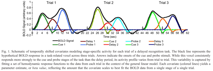 |
| Figure 1 from Rissman et al (2004). The caption is mostly self-explanatory, but note that for the beta-series correlation, we are looking at the amplitude estimates, or peaks of each waveform for each condition in each trial. Therefore, we would starting stringing together betas for each condition, and the resulting timecourse for, say, the Cue condition would be similar to drawing a line between the peaks of the first waveform in each trial (the greenish-looking ones). |
The first step to do this is to put each individual trial into your model; which, mercifully, is easy to do with AFNI. Instead of using the -stim_times option that one normally uses, instead use -stim_times_IM, which will generate a beta for each individual trial for that condition. A similar process can be done in SPM and FSL, but as far as I know, each trial has to be coded and entered separately, which can take a long time; there are ways to code around this, but they are more complicated.
Assuming that you have run your 3dDeconvolve script with the -stim_times_IM option, however, you should now have each individual beta for that condition output into your statistics dataset. The last preparation step is to extract them with a backhoe, or - if you have somehow lost yours - with a tool such as 3dbucket, which can easily extract the necessary beta weights (Here I am focusing on beta weights for trials where participants made a button press with their left hand; modify this to reflect which condition you are interested in):
3dbucket -prefix Left_Betas stats.s204+tlrc'[15..69(2)]'
As a reminder, the quotations and brackets mean to do a sub-brik selection; the ellipses mean to take those sub-briks between the boundaries specified; and the 2 in parentheses means to extract every other beta weight, since these statistics are interleaved with T-statistics, which we will want to avoid.
Tomorrow we will finish up how to do this for a single subject. (It's not too late to turn back!)
*Fensterwhacker, D. T. (2011). A Whale of a Night: An Investigation into the Neural Correlates of Listening to Whales Mating. Journal of Mongolian Neuropsychiatry, 2, 113-120.
**Unless you participate in one of my studies, of course.
Monday, May 19, 2014
Extracting and Regressing Out Signal in White Matter and CSF
A man's at odds to know his mind because his mind is aught he has to know it with. He can know his heart, but he don't want to. Rightly so. Best not to look in there.


-The Anchorite
==============
In the world of FMRI analysis, certain parts of the brain tend to get a bad rap: Edges of the brain are susceptible to motion artifacts; subcortical regions can display BOLD responses wholly unlike its cortical cousins atop the mantle; and pieces of tissue near sinuses, cavities, and large blood vessels are subject to distortions and artifacts that warp them beyond all recognition. Out of all of the thousands of checkered cubic millimeters squashed together inside your skull, few behave the way we neuroimagers would like.
Two of the cranium's worst offenders, who also incidentally make up the largest share of its real estate, are white matter and cerebrospinal fluid (CSF). Often researchers will treat any signal within these regions as mere noise - that is, theoretically no BOLD signal should be present in these tissue classes, so any activity picked up can be treated as a nuisance regressor.*
Using a term like "nuisance regressor" can be difficult to understand for the FMRI novitiate, similar to hearing other statistical argot bandied about by experienced researchers, such as activity "loading" on a regressor, "mopping up" excess variance, or "faking" a result. When we speak of nuisance regressors, we usually refer to a timecourse, one value per time point for the duration of the run, which represents something we are not interested in, or are trying to divorce from effects that we have good reason to believe actually reflect the underlying neural activity. Because we do not believe they are neurally relevant, we do not convolve them with the hemodynamic response, and insert them into the model as they are.
Head motion, for example, is one of the most widely used nuisance regressors, and are simple to interpret. To create head motion regressors, the motion in x-, y-, and z-directions are recorded at each timepoint and output into text files with one row per timepoint reflecting the amount of movement in a specific direction. Once these are in the model, the model will be compared to each voxel in the brain. Those voxels that show a close correspondence with the amount of motion will be best explained, or load most heavily, on the motion regressors, and mop up some excess variance that is unexplained by the regressors of interest, all of which doesn't really matter anyway because in the end the results are faked because you are lazy, but even after your alterations the paper is rejected by a journal, after which you decide to submit to a lower-tier publication, such as the Mongolian Journal of Irritable Bowel Syndrome.
The purpose of nuisance regressors, therefore, is to account for signal associated with artifacts that we are not interested in, such as head motion or those physiological annoyances that neuroimagers would love to eradicate but are, unfortunately, necessary for the survival of humans, such as breathing. In the case of white matter and CSF, we take the average time course across each tissue class and insert - nay, thrust - these regressors into our model. The result is a model where signal from white matter and CSF loads more onto these nuisance regressors, and helps restrict any effects to grey matter.
==============
To build our nuisance regressor for different tissue classes, we will first need to segment a participant's anatomical image. This can be done a few different ways:
1. AFNI's 3dSeg command;
2. FSL's FAST command;
3. SPM's Segmentation tool; or
4. FreeSurfer's automatic segmentation and parcellation stream.
Of all these, Freesurfer is the most precise, but also the slowest. (Processing times on modern computers of around twenty-four hours per subject are typical.) The other three are slightly less accurate, but also much faster, with AFNI clocking in at about twenty to thirty seconds per subject. AFNI's 3dSeg is what I will use for demonstration purposes, but feel free to use any segmentation tool you wish.
3dSeg is a simple command; it contains several options, and outputs more than just the segmented tissue classes, but the most basic use is probably what you will want:
3dSeg -anat anat+tlrc
Once it completes, a directory called "Segsy" is generated containing a dataset labeled "Classes+tlrc". Overlaying this over the anatomical looks something like this:
Note that each tissue class assigned both a string label and a number. The defaults are:
1 = CSF
2 = Grey Matter
3 = White Matter
To extract any one of these individually, you can use the "equals" operator in 3dcalc:
3dcalc -a Classes+tlrc -expr 'equals(a, 3)' -prefix WM
This would extract only those voxels containing a 3, and dump them into a new dataset, which I have here called WM, and assign those voxels a value of 1; much like making any kind of mask with FMRI data.
Once you have your tissue mask, you need to first resample it to match the grid for whatever dataset you are extracting data from:
3dresample -master errts.0050772+tlrc -inset WM+tlrc -prefix WM_Resampled
You can then extract the average signal at each timepoint in that mask using 3dmaskave:
3dmaskave -quiet -mask WM_Resampled+tlrc errts.0050772 > WM_Timecourse.1D
This resulting nuisance regressor, WM_Timecourse.1D, can then be thrust into your model with the -stim_files option in 3dDeconvolve, which will not convolve it with any basis function.
To check whether the average timecourse looks reasonable, you can feed the output from the 3dmaskave command to 1dplot via the-stdin option:
3dmaskave -quiet -mask WM_Resampled+tlrc errts.0050772 | 1dplot -stdin
All of this, along with a new shirt I purchased at Express Men, is shown in the following video.
*There are a few, such as Yarkoni et al, 2009, who have found results suggesting that BOLD responses can be found within white matter, but for the purposes of this post I will assume that we all think the same and that we all believe that BOLD responses can only occur in grey matter. There, all better.
Sunday, May 18, 2014
ReHo Normalization with FSL
As a brief addendum to the previous post, ReHo maps can also be normalized using FSL tools instead of 3dcalc. Conceptually, it is identical to what was discussed previously; however, the ability to set variables as the output of FSL commands makes it more flexible for shell scripting. For example, using the same datasets as before, we could set the mean and standard deviation to variables using the following combination of AFNI and FSL commands:
3dAFNItoNIFTI ReHo_Test_Mask+tlrc
3dAFNItoNIFTI mask_group+tlrc
setenv meanReHo `fslstats ReHo_Test_Mask.nii -M`
setenv stdReHo `fslstats ReHo_Test_Mask.nii -S`
fslmaths ReHo_Test_Mask.nii -sub $meanReHo -div $stdReHo -mul mask_group.nii ReHo_Norm
gunzip *.gz
3dcopy ReHo_Norm.nii ReHo_Norm
An explanation of these commands is outlined in the video below. Also, suits!
Friday, May 16, 2014
Regional Homogeneity Analysis, Part IV: Normalizing Correlation Maps
Once 3dReHo is completed and you have your correlation maps, you will then need to normalize them. Note that normalize can have different meanings, depending on the context. With FMRI data, when we talk about normalization we usually mean normalizing the data to a standard space so that individual subjects, with all of their weird-looking, messed-up brains, can be compared to each other. This results in each subject's brain conforming to the same dimensions and roughly the same cortical topography as a template, or "normal" brain, which in turn is based on the brain of an admired and well-loved public figure, such as 50 Cent or Madonna.
However, normalization can also refer to altering the signal in each voxel to become more normally distributed. This makes the resulting statistical estimates - whether betas, correlation coefficients, or z-scores - more amenable for a higher-level statistical test that assumes a normal distribution of scores, such as a t-test. Although there are a few different ways to do this, one popular method in papers using ReHo is to take the mean Kendall's Correlation Coefficient (KCC) of all voxels in the whole-brain mask, subtract that mean from each voxel, and divide by the KCC standard deviation across all voxels in the whole-brain mask.
As a brief intermezzo before going over how to do this in AFNI, let us talk about the difference between 3d and 1d tools, since knowing what question you want to answer will direct you toward which tool is most appropriate for the job. 3d tools - identified by their "3d" prefix on certain commands, such as 3dTfitter or 3dDeconvolve - take three-dimensional data for their input, which can be any three-dimensional dataset of voxels, and in general any functional dataset can be used with these commands. Furthermore, these datasets usually have a temporal component - that is, a time dimension that is the length of however many images are in that dataset. For example, a typical functional dataset may have several voxels in the x-, y-, and z-directions, making it a three-dimensional dataset, as well as a time component of one hundred or so timepoints, one for each scan that was collected and concatenated onto the dataset.
1d tools, on the other hand, use one-dimensional input, which only goes along a single dimension. The ".1D" files that you often see input to 3dDeconvolve, for example, have only one dimension, which usually happens to be time - one data point for every time point. Since we will be extracting data from a three-dimensional dataset, but only one value per voxel, then, we will use both 3d and 1d tools for normalization.
Once we have our regional homogeneity dataset, we extract the data with 3dmaskdump, omitting any information that we don't need, such as the coordinates of each voxel using the -noijk option:
3dmaskdump -noijk -mask mask_group+tlrc ReHo_Test_Mask+tlrc > ReHo_Kendall.1D
Note also that the -mask option is using the whole-brain mask, as we are only interested in voxels inside the brain for normalization.
The next step will feed this information into 1d_tool.py, which calculates the mean and standard deviation of the Kendall correlation coefficients across all of the voxels:
1d_tool.py -show_mmms -infile ReHo_Kendall.1D
Alternatively, you can combine both of these into a single using the "|" character will feed the standard output from 3dmaskdump into 1d_tool.py:
3dmaskdump -noijk -mask mask_group+tlrc ReHo_Test_Mask+tlrc | 1d_tool.py -show_mmms -infile -
Where the "-" after the -infile option means to use the standard output of the previous command.
3dcalc is then used to create the normalized map:
3dcalc -a ReHo_Test_Mask+tlrc -b mask_group+tlrc -expr '((a-0.5685)/0.1383*b)' -prefix ReHo_Normalized
Lastly, although we have used the whole brain for our normalization, a strong argument can be made for only looking at voxels within the grey matter by masking out the grey matter, white matter, and cerebrospinal fluid (CSF) separately using FreeSurfer or a tool such as 3dSeg. The reason is that the white matter will tend to have lower values for Kendall's correlation coefficient, and grey matter will have relatively higher values; thus, normalizing will bias the grey matter to have higher values than the grey matter and CSF. However, one could counter that when a second-level test is carried out across subjects by subtracting one group from another, it is the relative differences that matter, not the absolute number derived from the normalization step.
In sum, I would recommend using a grey mask, especially if you are considering lumping everyone together and only doing a one-sample t-test, which doesn't take into account any differences between groups. As with most things in FMRI analysis, I will leave that up to your own deranged judgment.
Monday, May 12, 2014
Regional Homogeneity Analysis, Part III: Running 3dReHo
Before moving on to using 3dReHo, we need to first ask some important rhetorical questions (IRQs):
This is demonstrated in the following video, which was recorded shortly before I was assaulted by my girlfriend with dental floss. Unwaxed, of course. (She knows what I like.)
- Did you know that with the advent of free neuroimaging analysis packages and free online databanks, even some hirsute weirdo like you, who has the emotional maturity of a bag full of puppies, can still do FMRI analysis just like normal people?
- Did you know that it costs ten times as much to cool your home with air conditioning than it does to warm it up?
- Did you know that Hitler was a vegetarian?
- Did you know that over thirty percent of marriages end by either knife fights or floss strangulation?
Once we have thought about these things long enough, we can then move on to running 3dReHo, which is much less intimidating than it sounds. All the command requires is a typical resting state dataset which has already been preprocessed and purged of motion confounds, as well as specifying the neighborhood for the correlation analysis; in other words, how many nearby voxels you want to include in the correlation analysis. For each voxel 3dReHo then calculates Kendall's Correlation Coefficient (KCC), a measure of how well the timecourse of the current voxel correlates with its neighbors.
3dReHo can be run with only a prefix argument and the input dataset (for the following I am using the preprocessed data of subject 0050772 from the KKI data analyzed previously):
3dReHo -prefix ReHoTest -inset errts.0050772+tlrc
The default is to run the correlation for a neighborhood of 27 voxels; that is, for each voxel touching the current voxel with either a face, edge, or corner. This can be changed using the -nneigh option to either 7 or 19. In addition, you can specify a radius of voxels to use as a neighborhood; however, note that this radius is in voxels, not millimeters.
E.g.,
3dReHo -prefix ReHo_9 -inset errts.0050772+tlrc -nneigh 9
Or:
3dReHo -prefix ReHo_rad3 -inset errts.0050772+tlrc -neigh_RAD 3
Lastly, if your current dataset has not already been masked, you can supply a mask using the -mask option, which can either be a whole-brain mask or a grey-matter mask, depending on which you are interested in. For the KKI dataset, which is not masked during the typical uber_subject.py pipeline, I would use the mask_group+tlrc that is generated as part of the processing stream:
3dReHo -prefix ReHo_masked -inset errts.0050772+tlrc -mask mask_group+tlrc
This is demonstrated in the following video, which was recorded shortly before I was assaulted by my girlfriend with dental floss. Unwaxed, of course. (She knows what I like.)
Sunday, May 11, 2014
Regional Homogeneity Analysis, Part II: Processing Pipelines
For regional homogeneity analysis (ReHo), many of the processing steps of FMRI data remain the same: slice-timing correction, coregistration, normalization, and many of the other steps are identical to traditional resting-state analyses. However, the order of the steps can be changed, depending on whatever suits your taste; as with many analysis pipelines, there is no single correct way of doing it, although some ways are more correct than others.
One of the most comprehensive overviews of ReHo processing was done by Maximo et al (2013), where datasets were processed using different types of signal normalization, density analysis, and global signal regression. I don't know what any of those terms mean, but I did understand when they tested how smoothness affected the ReHo results. As ReHo looks at local connectivity within small neighborhoods, spatial smoothing can potentially inflate these correlation statistics by averaging signal together over a large area and artificially increasing the local homogeneity of the signal. Thus, smoothing is typically done after ReHo is applied, although some researchers eschew it altogether.
So, should you smooth? Consider that each functional image already has some smoothness added to it when it comes directly off the scanner, and also that any transformation or movement of the images introduces spatial interpolation as well. Further, not all of this interpolations and inherent smoothness will be exactly the same for each subject. Given this, it makes the most sense to smooth after ReHo has been applied, but also to use a tool such as AFNI's 3dFWHMx to smooth each image to the same level of smoothness; however, if that still doesn't sit well with you, note that the researcher's from the abovementioned paper tried processing pipelines both with and without a smoothing step, and found almost identical results for each analysis stream.
Taken together, most of the steps we used for processing our earlier functional connectivity data are still valid when applied to a ReHo analysis; we still do the basic preprocessing steps, and still run 3dDeconvolve and 3dSynthesize commands to remove confounding motion effects from our data. However, we will only do smoothing after all of these commands have been run, and use 3dFWHMx to do it instead of 3dmerge.
One last consideration is the neighborhood you will use for ReHo. As a local connectivity measure, we can specify how much of the neighborhood we want to test for correlation with each voxel; and the most typical options are using immediate neighbors of 7, 19, or 27 voxels, which can be specified in the 3dReHo command with the -nneigh option. "7" will mean to consider only those neighboring voxels with one face touching; "19" will calculate the time-series correlation with any voxel touching with a face or an edge (e.g., a straight line bordering the current voxel); and "27" will do the analysis for any voxel with an abutting face, edge, or corner (think of it as the test voxel in the center of a Rubik's cube, and that voxel being correlated with every other voxel in the cube).

In the next part, we will go over some important rhetorical questions, along with a video showing how the command is done.
One of the most comprehensive overviews of ReHo processing was done by Maximo et al (2013), where datasets were processed using different types of signal normalization, density analysis, and global signal regression. I don't know what any of those terms mean, but I did understand when they tested how smoothness affected the ReHo results. As ReHo looks at local connectivity within small neighborhoods, spatial smoothing can potentially inflate these correlation statistics by averaging signal together over a large area and artificially increasing the local homogeneity of the signal. Thus, smoothing is typically done after ReHo is applied, although some researchers eschew it altogether.
So, should you smooth? Consider that each functional image already has some smoothness added to it when it comes directly off the scanner, and also that any transformation or movement of the images introduces spatial interpolation as well. Further, not all of this interpolations and inherent smoothness will be exactly the same for each subject. Given this, it makes the most sense to smooth after ReHo has been applied, but also to use a tool such as AFNI's 3dFWHMx to smooth each image to the same level of smoothness; however, if that still doesn't sit well with you, note that the researcher's from the abovementioned paper tried processing pipelines both with and without a smoothing step, and found almost identical results for each analysis stream.
Taken together, most of the steps we used for processing our earlier functional connectivity data are still valid when applied to a ReHo analysis; we still do the basic preprocessing steps, and still run 3dDeconvolve and 3dSynthesize commands to remove confounding motion effects from our data. However, we will only do smoothing after all of these commands have been run, and use 3dFWHMx to do it instead of 3dmerge.
One last consideration is the neighborhood you will use for ReHo. As a local connectivity measure, we can specify how much of the neighborhood we want to test for correlation with each voxel; and the most typical options are using immediate neighbors of 7, 19, or 27 voxels, which can be specified in the 3dReHo command with the -nneigh option. "7" will mean to consider only those neighboring voxels with one face touching; "19" will calculate the time-series correlation with any voxel touching with a face or an edge (e.g., a straight line bordering the current voxel); and "27" will do the analysis for any voxel with an abutting face, edge, or corner (think of it as the test voxel in the center of a Rubik's cube, and that voxel being correlated with every other voxel in the cube).
In the next part, we will go over some important rhetorical questions, along with a video showing how the command is done.
Friday, May 9, 2014
Regional Homogeneity Analysis with 3dReHo, Part 1: Introduction
Learning a new method, such as regional homogeneity analysis, can be quite difficult, and one often asks whether there is an easier, quicker method to become enlightened. Unfortunately, such learning can only be accomplished through large, dense books. Specifically, you should go to the library, check out the largest, heaviest book on regional homogeneity analysis you can find, and then go to the lab of someone smarter than you and threaten to smash their computer with the book unless they do the analysis for you.
If for some reason that isn't an option, the next best way is to read how others have implemented the same analysis; such as me, for example. Just because I haven't published anything on this method, and just because I am learning it for the first time, doesn't mean you should go do something rash, such as try to figure it out on your own. Rather, come along as we attempt to unravel the intriguing mystery of regional homogeneity analysis, and hide from irate postdocs whose computers we have destroyed. In addition to the thrills and danger of finding things out, if you follow all of the steps outlined in this multi-part series, I promise that you will be the first one to learn this technique from a blog. And surely, that must count for something.
With regional homogeneity analysis (or ReHo), researchers ask similar questions as with functional connectivity analysis; however, in the case of ReHo, we correlate the timecourse in one voxel with its immediate neighbors, or with a range of neighbors within a specified radius, instead of using a single voxel or seed region and testing for correlations with every other voxel in the brain, as in standard functional connectivity analysis.
As an analogy, think of ReHo as searching for similarities in the timecourse of the day's temperature between different counties across a country. One area's temperature timecourse will be highly correlated with neighboring counties's temperatures, and the similarity will tend to decrease the further away you go from the county you started in. Functional connectivity analysis, on the other hand, looks at any other county that shows a similar temperature timecourse to the county you are currently in.
Similarly, when ReHo is applied to functional data, we look for differences in local connectivity; that is, whether there are differences in connectivity within small areas or cortical regions. For example, when comparing patient groups to control groups, there may be significantly less or significantly more functional connectivity in anterior and posterior cingulate areas, possibly pointing towards some deficiency or overexcitation of communication within those areas. (Note that any differences found in any brain area with the patient group implies that there is obviously something "wrong" with that particular area compared to the control group, and that the opposite can never be true. While I stand behind this arbitrary judgment one hundred percent, I would also appreciate it if you never quoted me on this.)
As with the preprocessing step of smoothing, ReHo is applied to all voxels simultaneously, and that the corresponding correlation statistic in each voxel quantifies how much it correlates with its neighboring voxels. This correlation statistic is called Kendall's W, and ranges between 0 (no correlation at all between the specified voxel and its neighbors) and 1 (perfect correlation with all neighbors). Once these maps are generated, they can then be normalized and entered into t-tests, producing similar maps that we used with our functional connectivity analysis.
Now that we have covered this technique in outline, in our next post we will move on to the second, more difficult part: Kidnapping a senior research assistant and forcing him to do the analysis for us.
No, wait! What I meant was, we will review some papers that have used ReHo, and attempt to apply the same steps to our own analysis. If you have already downloaded and processed the KKI data that we used for our previous tutorial on functional connectivity, we will be applying a slightly different variation to create our ReHo analysis stream - one which will, I hope, not include federal crimes or destroying property.
Subscribe to:
Posts (Atom)